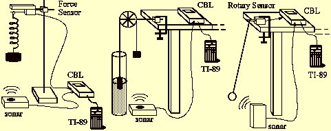
To study oscillatory motions with on-line apparatuses (sensors + interface + calculator) may be quite exciting. In fact the system evolution in time becomes directly accessible in a quantitative way. Plots of position, velocity and acceleration versus time allow an immediate evaluation of the essential characteristics of the observed motion. Also the experimental investigation within less common graphic representations (velocity/position, acceleration/position, force/acceleration, force/position …) may offer precious hints for a deeper understanding.To illustrate the potentialities the on-line experiments, we consider here 3 oscillating systems: two of them being normally part of introductory courses in mechanics (mass-spring and pendulum), while the third (an Atwood machine with one of the masses in water bath) is less common but well suited to show the transition from harmonic to anharmonic behavior, an aspect often neglected in the traditional laboratory. The mass-spring oscillator (obeying to Hooke’s law) is always harmonic, the Atwood oscillator evolves from anharmonic at large amplitude to harmonic at small amplitude (the Archimedes’ + gravitational restoring force switches from a constant value to values proportional to displacement when the mass is partially submerged in water) while in the case of pendulum the intrinsically anharmonic motion may be approximated to harmonic motion in the limit of small amplitude.

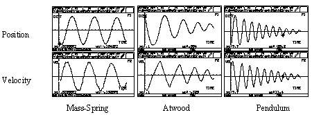
The position vs. time plots x(t) are quite similar: at first sight they look like sinusoids, more or less damped. However the velocity vs. time plots v(t) show evident differences in the 3 oscillators. In the mass-spring harmonic oscillator the velocity plot is the same as the position plot, with a phase leading of 90°. In the Atwood oscillator the velocity plot, at large amplitude, is made of straight segments, showing that the motion is uniformly accelerated, with acceleration changing sign at each half-period, while at small amplitude it recall the mass-spring behavior. Also the large amplitude oscillations of the pendulum is far from sinusoidal: you can’t see it in the x(t) plot, but you’ll see it well in the v(t) plot, and even better in the a(t) plot.The availability of the whole data set, and not only of few of them (e.g. those related to gate crossing, as in the traditional laboratory) allows this qualitative but important analysis .Harmonicity implies isochronism. A quantitative analysis of the plots yields immediately the period as a function of amplitude that allows to test the predictions of models for different non-linear restoring forces.

Eight sessions of laboratory demonstrations are scheduled during the Physics Olimpiad in Padua, where many other experiments on oscillations will be performed using a simple on-line apparatus (Galileo oscillator, Maxwell wheel, chart on incline, see-saw on round or square pivot…)

The majority of the phenomena are intrinsically anharmonic motions, as most of the ordinary-life mechanical oscillations. This is due to the fact that usually the restoring force is produced by some component of the gravity field, which is constant. In some cases a quasi harmonic motion may be obtained by choosing a proper system geometry (pendulum) and small departures from equilibrium position. Intrinsically harmonic motion is produced only by a restoring force which is linearly dependent on the displacement, as in the case of mass-spring oscillator, or of the Atwood oscillator (when the immersed body has uniform cross section).